From One Oscillator to Many

Algebra is just easier than solving partial differential equations

The irreducible representations anyway. This is a consequence of the Stone von Neumann theorem, which we can discuss at length later one.

Yet Another Representation of the Heisenberg Algebra

The algebra we have been working with involves a three-dimensional vector space 𝔥 spanned by the operators a, a† and 1. The only nontrivial commutator is

\([a,a^{\dagger}] = 1.\)

In the past two installments we’ve studied how this algebra comes from Quantum Mechanics of the simple harmonic oscillator.

There is another representation of this same algebra which is fairly intuitive, spanned by the operators¹

\(z, \; \frac{d}{dz}\; \mathrm{and} \; 1.\)

These operators can act on differentiable functions of the variable z, as for any given differentiable function of f(z)

\(z f(z),\; \frac{df(z)}{dz}\;\mathrm{and}\; 1\cdot f(z)\)

are all also differentiable functions of the variable z.

They are also all linear operators in the sense that they preserve the structure of linear combinations, for example,

\(\frac{d}{dz}\left(af(z) + b g(z)\right) = a\frac{df(z)}{dz} + b\frac{dg(z)}{dz}.\)

where a and b are constants and f and g are any two differentiable functions of z.

We can therefore compute the commutators of these linear operators,

\(\left[\frac{d}{dz},z\right]f(z) = f(z) + z\frac{df(z)}{dz} - z\frac{df(z)}{dz} = f(z).\)

which we can just write as

\(\left[\frac{d}{dz},z\right] = 1.\)

Hence we have an isomorphism with our other algebra 𝔥,

\(a \leftrightarrow \frac{d}{dz},\; a^{\dagger} \leftrightarrow z,\; 1 \leftrightarrow 1.\)

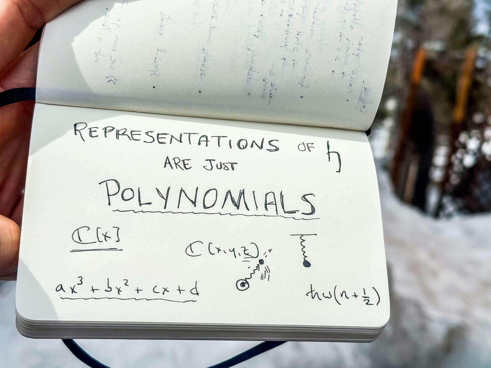
Polynomials represent The Heisenberg Algebra

While we know that this new algebra acts on differentiable functions we can be more precise than that. The simplest representation for this algebra the we can write down is given by the vector space of complex polynomials² in z, C[z].

Under the above algebra isomorphism, its action on C[z] is isomorphic to the former’s action on the vector space of physical states³,

\(\Omega \leftrightarrow 1,\quad v_{n} \leftrightarrow z^{n}.\)

Hence a generic polynomial in z corresponds to a generic member of the representation.

Notice that the energy operator in this representation is given by

\(E = \hbar\omega\left( z\frac{d}{dz} + \frac{1}{2}\right).\)

As expected, the monomials in C[z] correspond to energy eigenstates,

\(E\cdot z^{m} = \hbar\omega\left( m + \frac{1}{2}\right)\,z^{m}.\)

From a Mathematicians point of view, we can strip that energy operator down to the so-called degree operator⁴,

\(N = z \frac{d}{dz}.\)

And hence each monomial in z spans a one-dimensional linearly independent subspace with distinct degree. These correspond to the excitation level of the physical system - otherwise modeled as the amplitude of oscillations.

This theme of vector spaces as polynomials in raising or creation operators will be ubiquitous throughout our study of Heisenberg algebras, Quantum Field Theory and Vertex Operator Algebras.

The Upshot of Polynomial Representations

Our new representation started with the study of differentiable functions, but we’ve ended up with a representation of polynomials. Of course, these are related. Analytic functions are precisely those which have power series representations, they’re also the kind of function that physicists typically have in mind when study physical phenomena⁵.

More broadly, physicists often invoke Taylor’s theorem to find a suitable approximation of physical phenomena with polynomials where appropriate.

In two-dimensional conformal field theory, complex analytic functions are precisely those which enjoy (local) conformal symmetry, and hence all such quantum fields are essentially modeled by a power series representation.

A Rapid, Intuitive Generalization to Three-Dimensions

In algebraic form, this algebra generalizes without much difficulty. Let 𝔥[z] be the algebra spanned by our three operators

\(z,\quad \frac{d}{dx},\quad 1.\)

Then 𝔥[x,y,z] can be written in terms of the seven operators

\(x, y,z,\;\partial_{x},\partial_{y},\partial_{z},\; 1.\)

You can immediately identify three isomorphic subalgebras, 𝔥[x],𝔥[y] and 𝔥[z], which each act upon their own vector space of states,

\(\mathbb{C}[x],\quad \mathbb{C}[y],\quad \mathbb{C}[z],\)

respectively.

The three individual subalgebras all commute amongst themselves. We can write this collectively as

\(\left[\mathfrak{h}[x],\mathfrak{h}[y]\right] = \left[\mathfrak{h}[y],\mathfrak{h}[z]\right] = \left[\mathfrak{h}[z],\mathfrak{h}[x]\right] = 0.\)

The only relevant commutators in the full algebra are

\([\partial_{x},x] = [\partial_{y},y] = [\partial_{z},z] = 1.\)

It’s easy to see then that the full algebra acts on the product of these three vector spaces of polynomials,

\(\mathbb{C}[x,y,z] \cong \mathbb{C}[x]\otimes\mathbb{C}[y]\otimes\mathbb{C}[z].\)

That is to say, it acts on the vector space of polynomials in all three variables, x, y and z.

We immediately have the vector space of physical states without having to solve a complicated system of three-dimensional, second order, partial differential equations⁶.

Assuming we have isotropic coordinates, the energy operator for this representation can be given as

\(E = \hbar\omega\left( x\partial_{x} + y\partial_{y} + z\partial_{z} + \frac{3}{2}\right).\)

and the degree operator is

\(N = x\partial_{x} + y\partial_{y} + z\partial_{z}.\)

What’s novel about the three-dimensional oscillator is that there are linearly independent physical states that share the same energy eigenvalues.

N = 1

The obvious case are the three monomials of unit degree,

\(x,y,z,\quad E = \frac{5}{2}\hbar\omega.\)

N=2

There are six monomials of degree 2,

\(x^{2},y^{2},z^{2},xy,yz,xy\quad \Rightarrow E = \frac{7}{2}\hbar\omega.\)

And so on. What’s amusing about this construction is that the mathematics is analogous⁷ to that three independent, one-dimensional harmonic oscillators.

This immediately suggests a problem in Statistical Mechanics.

Grading our Vector Spaces: The case of n-oscillators.

Let n be a finite, positive integer. Consider an ensemble of n distinct⁸, one-dimensional simple harmonic oscillators. We immediately know that the space of states associated to this system is the vector space of polynomials in n variables. Let V be this vector space,

\(V = \mathbb{C}[x_{1},x_{2},\cdots,x_{n}].\)

For the case of n=1, we’ve already seen that this vector space C[z] separates into one-dimensional subspaces of fixed degree, spanned by basis vectors

\(1, z, z^{2},\cdots , z^{n}, z^{n+1},\cdots .\)

For generic n, these subspaces are easy to define, although their dimensions grow rapidly with degree. We can decompose V as a the direct sum of subspaces by degree,

\(V \cong \bigoplus_{k=0}^{\infty} V_{k},\)

where V_k contains all the monomials in V of degree k.

By the way, any vector space that can be decomposed into the direct sum of subspaces with fixed degree is said a graded vector space, and in particular, is graded by the set of those degrees. For example, our module V is graded by the natural numbers, N, as it can be written as the direct sum of subspaces V_k that enjoy a fixed degree, k.

For example, if n = 3

\(x^{4},\;x^{3}y, \;x^{2}yz,\;x^{2}z^{2} \in V_{4}\)

are all monomials of degree four. In total there are 15 such terms that span V_4. Another term for V_k would be the homogeneous polynomials of degree 4.

Generally, the the dimension of V_k scales with both k and n,

\(\dim V_{k} = \left(\begin{array}{c}n+k-1 \\ k\end{array}\right) = \frac{n(n+1)(n+2)\cdots (n+k-1)}{k!}.\)

A slight generalization of this approach - where frequency of oscillation for each oscillator was distinct⁹ - is essentially how Max Planck derived his formula for blackbody radiation - the spectrum of thermal radiation inside a oven at fixed temperature¹⁰, which eventually formalized our notion of the physical constant ℏ.

Appendix: The Three-Dimensional Harmonic Oscillator

The main distinction between three equivalent one-dimensional harmonic oscillators and a single, three-dimensional harmonic oscillator is the kinetic energy. In three dimensions we have to worry about rotational motion. Exciting oscillations in multiple directions will certainly induce angular motion.

The energy operator in three-dimensional, spherical polar coordinates is given by,

\(E = -\frac{\hbar^{2}}{2m}\frac{d^{2}}{dr^{2}} + \frac{\hbar^{2}}{2mr^{2}}\ell(\ell+1) + \frac{1}{2}m\omega^{2}r^{2},\)

where r is the radial coordinate and ℓ(ℓ+1) is the eigenvalue associated to the total angular momentum operator, and ℓ is restricted to nonnegative integers¹¹.

In this functional representation, the quantum states take on rather complicated¹² solutions Ψ_(n,ℓ,μ), indexed by three integers, n, ℓ and μ.

The energy operator in this representation has eigenvalues

\(E\cdot \psi_{n,\ell,\mu} = \hbar\omega\left(2n+ \ell + \frac{3}{2}\right)\;\psi_{n,\ell,\mu}.\)

Here both n, ℓ are nonnegative integers, and it is easy to see that the sum (2n+ℓ) is also. The other integer μ takes all integer values between -ℓ and ℓ, and corresponds to the other quantum states with the same total angular momentum, just distributed amongst the various dimension¹³. μ is not present in the energy eigenvalues precisely because the potential itself is spherically symmetric, and so does not depend on any particular angular direction. Hence there are multiple quantum states with identical energy eigenvalues. More precisely, for fixed n and ℓ, there are 2ℓ+1 of them.

Let’s look at some basic examples of how the three-dimensional functional representation of the three-dimensional oscillator corresponds with our algebraic representation.

Degree (2n+ℓ) = 1

Here exciting the ℓ = 1 mode corresponds to exciting a single mode of angular momentum, such as the state¹⁴

\(\psi_{0,1,0}(r,\theta,\phi) \rightsquigarrow z\cdot \Omega.\)

As just discussed, we would expect 3 distinct states with energy eigenvalues. Hopefully it’s clear that these are given by

\(\psi_{0,1,-1}(r,\theta,\phi) \rightsquigarrow (x+y)\cdot \Omega,\quad \psi_{0,1,1}(r,\theta,\phi) \rightsquigarrow (x-y)\cdot \Omega.\)

Degree (2n+ℓ) = 2

Here we have two possibilities: either (n = 1 and ℓ = 0) or (n = 0 and ℓ = 2). In the former case, μ is fixed at zero. In the latter case, there are five distinct values of μ. This gives us a total of six states.

In terms of C[x,y,z], the vector space of degree two is spanned by the six operators

\(x^{2},\,y^{2},\,z^{2},\,xy,\,yz,\,zx.\)

The n = 1 mode is actually a symmetric linear combination of all three squares,

\(\psi_{1,0,0} \rightsquigarrow \left(x^{2} + y^{2} + z^{2}\right).\)

All others are distributed amongst the other five states of degree two,

\(\psi_{0,2,-2},\,\psi_{0,2,-1},\,\psi_{0,2,0},\,\psi_{0,2,1},\,\psi_{0,2,2}.\)

Further excitations can be understood in terms of further combinations of the operators x, y and z on the vacuum Ω.

In short, it’s the same representation. Connections to specific physical phenomena, such as angular momentum require a more precise treatment to find the precise isomorphism of the two representations.

1. Note that this is a different representation from the one used by physicists in the study of the Schrödinger equation. It’s a linear combination akin to a 45 degree rotation of the physical position and momentum operators.

2. Here we are using boldface C to represent the field of complex numbers, and hence C[z] are the polynomials in z.

3. For details and definitions, check out our previous post:

4. Physicists will often call the corresponding N = a†a the number operator.

5. At least within a specific domain. Boundary conditions can abruptly change phenomena and often a function is not differentiable at a boundary. Piecewise smooth functions might be a safer representation, but it’s important to keep in mind that these are all just models.

6. This assumes that the restorative force that pulls the mass back towards the origin is isotropic. If it isn’t, we can typically choose coordinates so that it is. In general, the potential energy function will involve a generic, quadratic polynomial in all three spatial coordinates. We can always find a choice of coordinates that will have at least one and at most three diagonal harmonic oscillator potentials, up to an overall constant term. If you don’t have all three dimension represented, congratulations! You have one or more free particle directions that can be solved by simple plane waves. But for the sake of this piece, let’s retain our focus on the three dimensional oscillator.

7. As usual with degenerate physical states, observation can force a linear combination which might be in a more complicated basis. See the appendix at the end of this post for more details.

8. The word distinct is doing a lot of work here. Let us set them up so they’re all a different color, or spatially separated in such a way that there is no possible way to confuse one from the other.

9. This would certainly guarantee that the oscillators could be independently distinguished from the perspective of Quantum Mechanics!

10. See for example §7.2 of Pathria’s Statistical Mechanics.

11. Here we have already carried out the relevant decomposition of the eigenfunction in terms of spherical harmonics, avoiding the angular derivatives altogether. For a full accounting of the three-dimensional solution, check out any standard textbook on Quantum Mechanics.

12. As with the one-dimensional case, this is essentially an extension of the Gaussian function - this time as a function of the radical coordinate - together with some normalization factors and the associated Laguerre polynomials.

13. Understanding this point thoroughly is yet another good reason to study the details of the three-dimensional Schrödinger equation in any standard textbook.

14. We are being schematic here, our variables x,y and z do not correspond to the usual components in three-dimensional space time.