The Physical Origins of Heisenberg Algebras

Our first in a series of lectures on vertex operator representations of affine sl2.

Greetings!

It has become apparent that my original lecture notes associated with our video study of vertex operator algebras on YouTube have gone missing. To make up for that, I’ve started rewriting them, and will post them here. They should also serve as a nice lead up to another set of videos, focusing on the untwisted vertex operator realizations of affine sl2C.

Vertex Operator Algebras are effectively the same thing as two-dimensional conformal field theories¹, and are hence related to string theory. Indeed, the vertex operator itself is modeled on interactions from the world sheet perspective.

The representation theory of affine sl2C essentially amounts to the study of a bosonic string propagating on the SL2C group manifold - anomaly and related issues not withstanding.

We’re going to start from the physicists perspective, which means we’ll be highly informal for the first few lectures, and try to use that tone to pull as many of you folks along as we can.

We will come back to add formality and character to these early discussions much later, but it will be worth keep your representation theorist hat on while reading them, even if it’s messy. In some sense, it’s nice to see exactly where algebraic techniques can help make the physical ideas more precise.

Best,

Sean

---

The Simple Harmonic Oscillator

The simple harmonic oscillator is a toy model that has profound application across physical disciplines. It’s essentially an object of mass 𝑚 subject to a linear restorative force that induces oscillations of angular frequency 𝜔 when disturbed. That is to say,

\(q(t) \propto \cos(\omega t).\)

What’s novel about a linear restorative force is that the energy is essentially related to the amplitude of oscillations. The oscillation frequency is dictated by the material properties of the physical system. If 𝑝 is the associated momentum, then the energy is

\(E = \frac{p^{2}}{2m} + \frac{1}{2}m\omega^{2}q^{2}.\)

This is just a quadratic form on the symplectic vector space known to Physicists as phase space.

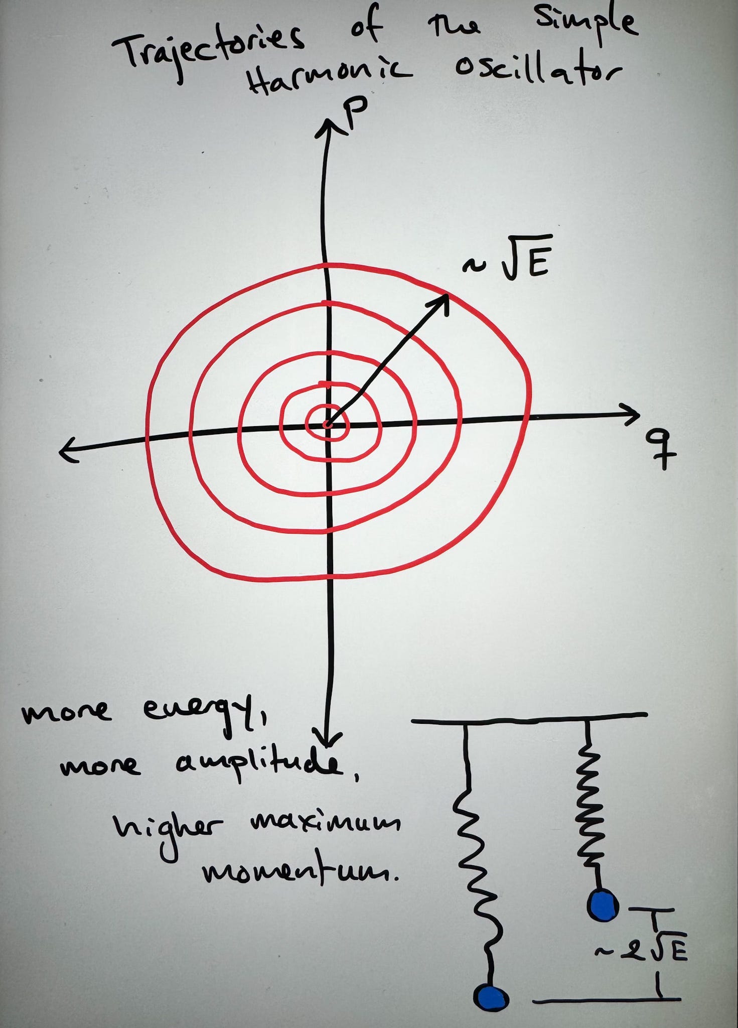
Classical motion corresponds to curves in phase space, and in this case - for suitably normalized coordinates - these are concentric rings about the origin.

In this case the energy is a constant of motion which dictates the amplitude of the oscillation. For the classical oscillator, a zero energy state involves no motion. This is represented by the point at the origin.

For real physical systems, this structure breaks down at sufficiently high energy - the spring may deform or break, for example. Dissipative forces such as air resistance also cause the system to slowly spiral towards the zero energy state. For small oscillations around a stable equilibrium, this is a reasonable model.

Trajectories of the point mass form concentric, nonintersecting loops. If we choose appropriate units, these are concentric circles. The amplitude of oscillations in either p or q then would be the radius whose value scales with the square root of energy.

This model is considered linear in the sense that the restoring force is directly proportional to the displacement

\(F = - kq.\)

Hooke’s constant of proportionality is related to the angular frequency of motion - and the object’s mass - via

\(\omega = \sqrt{\frac{k}{m}},\)

as can be readily verified by studying the physical system in detail.

Before moving to the study of the quantum version of this system, it’s worth highlighting two things. First, the main observables we can study the system with are position and momentum. Having made observations of p and q at various times we can interpolate to figure out what the energy is. The energy determines the trajectory - that loop in phase space - which is the physical state of the oscillator.

The Simple Heisenberg Algebra, 𝔥

In Classical Mechanics, energy is a continuous variable. In Quantum Mechanics, this no longer needs to be true. Quantum Mechanics introduces a noncommutative algebra in phase space,

\(qp - pq = i\hbar,\)

parametrized by the physical constant ℏ.

Following Dirac², we may change variables,

\(\eta = \sqrt{\frac{m\omega}{2\hbar}}\left(q + \frac{i}{m\omega}p\right),\quad \bar{\eta} = \sqrt{\frac{m\omega}{2\hbar}}\left(q - \frac{i}{m\omega}p\right).\)

The commutator of these new variables gives a simpler relation,

\(\eta\bar{\eta} - \bar{\eta}\eta = -\frac{2i}{2\hbar}\left(qp - pq\right) = 1.\)

In this language we find the energy to be written as,

\(E = \frac{\hbar\omega}{2}\left(\eta\bar{\eta} + \bar{\eta}\eta\right).\)

These are both manifestation of the same Lie algebra. It is the nontrivial nilpotent Lie algebra of smallest dimension. To refresh yourself on what that means, check out one of our older posts.

For a three-dimensional vector space 𝔥, spanned by 𝑥, 𝑦, 𝑧, the singular nontrivial Lie bracket is

\([x,y] = z.\)

This highlights the main structure of Quantum Theory:

Physical observables correspond to linear operators on a Hilbert space of physical states.

Determining which operators and what space of states they are represented on is part of the Art of this Science. It’s also - in my view - part of the reason that algebraic approaches to Quantum Mechanics can clarify the physics.

That was very abstract. Let’s get concrete.

The Functional Representation of 𝔥

Textbook Quantum Mechanics usually begins with the identifications

\(q \rightsquigarrow x,\quad p \rightsquigarrow -i\hbar\frac{d}{dx}.\)

so that

\([q,p] \rightsquigarrow i\hbar [x,\frac{d}{dx}] = i\hbar.\)

Implicitly this creates a module³ for 𝔥 out of the differentiable, complex functions in the variable x, which itself is assumed to represent the position of the system.

Function spaces are of course vector spaces, for if a and b are any two constants, and f(x) and g(x) are two two functions, then so too is a f(x) + b g(x).

Perhaps you can see the vagueness of a functional representation. What kind of functions are we talking about? Should they be smooth functions, if not how many times differentiable will do? Are they bounded functions? How are they bounded if so?

For better or worse, the Physicist’s response to these concerns typically involves boundary conditions and eye-rolling. In particular, we simply impose this representation on the energy operator

\(E \rightsquigarrow -\frac{\hbar^{2}}{2m}\frac{d^{2}}{dx^{2}} + \frac{1}{2}m\omega^{2}x^{2},\)

and assert that physically observable states are the eigenfunctions of this operator, whose associated energies are the corresponding eigenvalues.

A generic state then can the be represented as complex-linear combinations of these eigenfunctions. Such a state is called a wavefunction, which happens to serve something akin to an integration kernel for a probability distribution⁴.

Fortunately, the associated differential equation for the energy of a simple harmonic oscillator has well-known classical solutions based on the Hermite Polynomials. Hence we are presented with a complete, orthonormal basis for the vector space of square-summable⁵ functions. So we get an irreducible representation of 𝔥 thanks to the hard, detail intensive work of 19th century mathematicians.

Put differently, you either have to study the functional analysis to convince yourself - or close your eyes an invoke the relevant theorems - to arrive at the basis of physical states indexed by an positive integer n,

\(\psi_{n}(x) = \frac{1}{\sqrt{2^{n}n!}}\left(\frac{m\omega}{\pi\hbar}\right)^{1/4} \exp{\left(-\frac{m\omega x^{2}}{2\hbar}\right)}H_{n}\left(\sqrt{\frac{m\omega}{\hbar}}x\right).\)

Stare at that function for a second. The first two factors are a normalization constant. The third is a Gaussian function, whose normalization you might also consider when looking back at the second. The fourth factor is a polynomial H_n of order n - with integral coefficients - which also happens to be an even or odd function of x. Hence so is ψn(x).

As a unified whole, you can think of these functions as generalizations of the Gaussian function to include n+1 local extrema.

These eigenfunctions happen to be normalized so that

\(\int_{\mathbb{R}} \overline{\psi}_{m}\psi_{n}\, dx = \delta_{mn}.\)

You are welcome to derive or look up the Hermite Polynomials yourself, and can hence verify that the energy eigenvalues which solve the eigenvalue equation,

\(E \cdot \psi_{n} = E_{n}\psi_{n},\)

are given by

\(E_{n} = \hbar\omega\left(n + \frac{1}{2}\right).\)

Hence we see that where energy was previously a continuous parameter of our physical system, in the Quantum description, energy takes discrete values. This is a generic feature of so-called bound states, at least in one-dimension.

In particular, notice that the lowest energy state no longer has zero energy.

In physical problems where the potential energy function has a maximum finite value, we have two distinct series of representations. The bound states form a discrete series - not unlike our simple harmonic oscillator. The free states have a continuous series, parametrized by the energy. Bound states all occur below a threshold binding energy - the effectively the maximum of the potential energy function, and free states occur above it.

This distinction is common in representation theory, writ large.

Next Time

We’ll follow Dirac’s path to a much cleaner - but isomorphic - representation of 𝔥 and the related physics.

1. At least, the chiral half of homomorphically factorizable, two-dimensional CFTs.

2. For the most part in this essay we use Dirac’s original notation from his textbook.

3. A module is vector space upon which a Lie algebra acts. For our purposes its essentially the same as a representation, we’ll get into those details later on in the series.

4. We won’t delve too deeply into the axioms of Quantum Mechanics, but suffice it to say, physical observables are operators on a Hilbert space of physical states or wavefunctions. Nature is assumed to be inherently stochastic, and the expectation values of the aforementioned physical observables corresponding to appropriate use of their associated operators in conjunction with modulus square of the wavefunction as kernel. To be a bit more precise without starting a new lecture, observations may only be made of a specific eigenvalue for a given operator. Which eigenvalue is chosen at random.

5. That is to say, integrable. There is a little nuance as the Hermite polynomials form a basis when used with a Gaussian kernel, but this kernel is wrapped up into the definition of the physical eigenfunctions and doesn’t change representation at all.