Dirac's Algebraic Hilbert space.

Algebra can be much easier than Functional Analysis

Hey Friends,

This is our second installment in a set of lecture notes that will build towards the vertex operator representations of affine sl2C. Because we’re beginning with the physics, our first few lectures less formal than usual. Hang in there! We’ve got a bit more ground to cover before we let the Bourbaki zambonis loose.

Sean

---

Last time, we found the simple¹, three-dimensional Heisenberg algebra hiding the Quantum Mechanics of the simple harmonic oscillator:

We also learned some physics! We saw that the classical trajectories of a mass on a string could be represented by concentric circle in phase space. The radius of these circles - these orbits - scaled with the energy of the system.

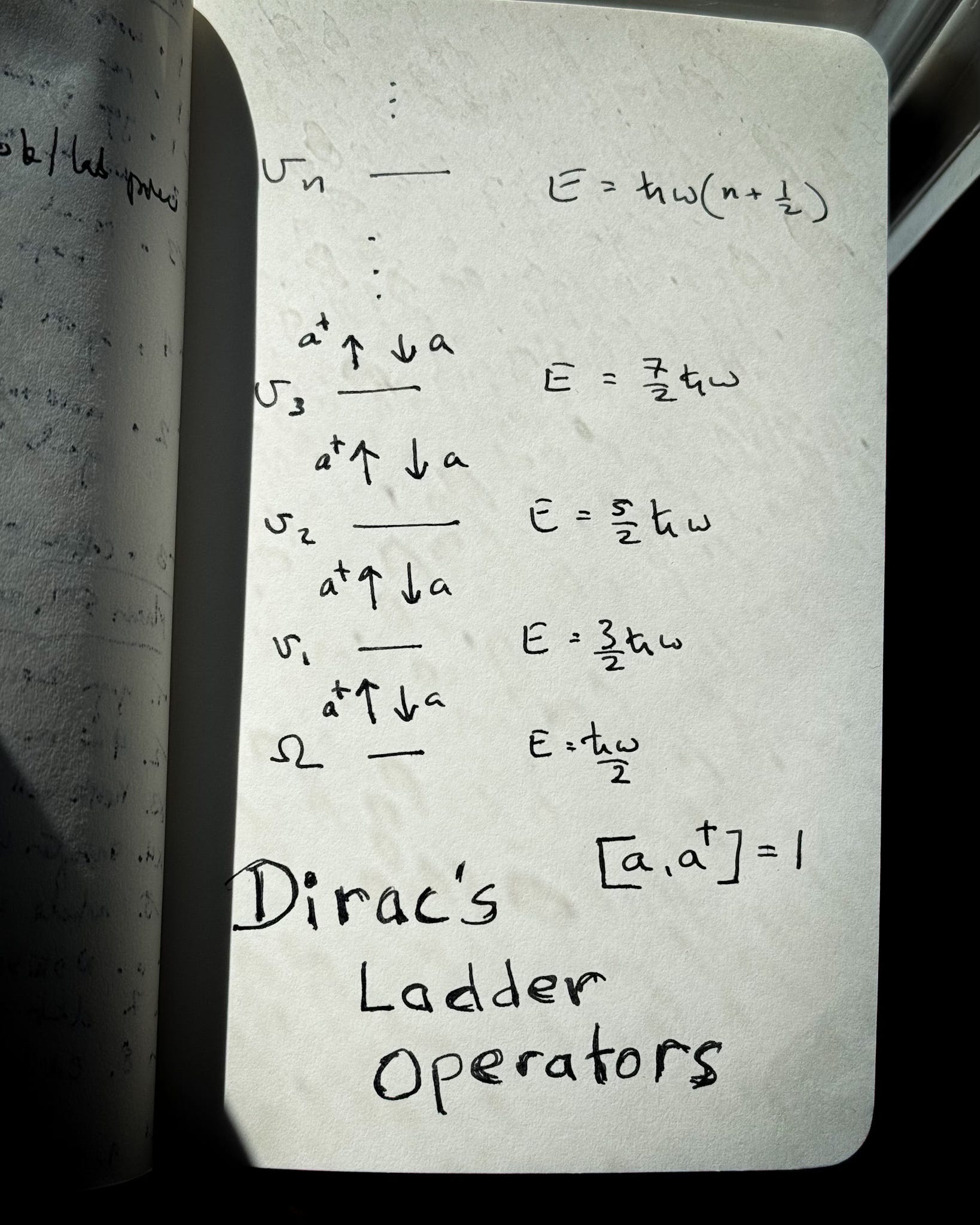
In the quantum case, these orbits were quantized to discrete values of energy,

\(E_{n} = \hbar\omega\left(n + \frac{1}{2}\right).\)

where n was any nonnegative integer. These integers label the linearly independent states of the physical system.

In Quantum Mechanics, the physical state of the system is represented by a vector space with a positive definite inner product, what some call a Hilbert space. The inner product of a Hilbert space can be used to define a norm - a notion of distance from the zero vector.

Let H be such a Hilbert space that models the simple harmonic oscillator detailed above. Evidently, H is countably² infinite-dimensional.

Physical observables then correspond to linear maps from H to itself. We often refer to these as linear operators on H. From a mathematician’s perspective, the algebra of these linear operators form a representation of that algebra on H³.

Much of the struggle for interpreting what the physicists mean by a “Hilbert space” stems from the fact that they typically don’t specify what vector space - or even what kind of vector space - the physical states exist in until after they’ve solved for the eigenvalues of the energy operator.

We will remedy this situation in due course.

A change of basis for 𝔥

Recall that the algebra of operators associated to the harmonic oscillator involved the commutator

\([q,p] = i\hbar.\)

Here here ℏ is a physical constant and i is the imaginary unit. Let us reconsider the linear combinations of the observables p and q, represented by the linear operators

\(q \rightsquigarrow x,\quad p \rightsquigarrow -i\hbar\frac{d}{dx}.\)

In this basis we can switch to our alternative coordinates⁴,

\(\eta \rightsquigarrow a = \sqrt{\frac{m\omega}{2\hbar}}\left(x + \frac{\hbar}{m\omega}\frac{d}{dx}\right),\quad \bar{\eta}\rightsquigarrow a^{\dagger} = \sqrt{\frac{m\omega}{2\hbar}}\left(x - \frac{\hbar}{m\omega}\frac{d}{dx}\right)\)

We’ll spare you the gory details, but it’s worth comparing the above operators to the simple commutator

\(\left[ x + \frac{d}{dx} , x - \frac{d}{dx}\right] = 2\left[\frac{d}{dx},x\right] = 2.\)

You can verify all the factors of two yourself to see that

\([a,a^{\dagger}] = 1.\)

And so we essentially have a linear transformation to a new basis of operators representing the same algebra.

Note also that the energy operator in this representation can be written

\(E = \frac{\hbar\omega}{2}\left(aa^{\dagger} + a^{\dagger}a\right)= \hbar\omega \left( a^{\dagger}a + \frac{1}{2}\right).\)

A Pair of Propositions

You can treat these as exercises if you like.

Proposition 1:

\([a,a^{\dagger n}] = na^{\dagger n-1}.\)

Proof.

We prove by induction. First observe by definition that this statement is true for n=1. Next assume it is true for some n. Then we compute,

\([a,a^{\dagger n+1}] = aa^{\dagger n+1} - a^{\dagger n+1}a = a^{\dagger n}a a^{\dagger} + [a,a^{\dagger n}]a^{\dagger} -a^{\dagger n-1}a.\)

Applying the assumption,

\([a,a^{\dagger n+1}] = a^{\dagger n+1}a + a^{\dagger n}[a,a^{\dagger}] + na^{\dagger n} - a^{\dagger n+1}a = (n+1)a^{\dagger n}.\)

The proposition follows by induction. ■

Proposition 2:

\([a^{\dagger}a,a^{\dagger n}] = n a^{\dagger n}.\)

Proof.

First we have

\([a^{\dagger}a , a^{\dagger n}] = a^{\dagger}aa^{\dagger n} - a^{\dagger n+1}a = a^{\dagger}[a,a^{\dagger n}].\)

The proposition follows from proposition 1. ■

Dirac’s Considerably Less Tedious Representation of 𝔥

Dirac’s big insight came from the realization that the ground state⁵ of the quantum harmonic oscillator was in the kernel⁶ of the linear operator a,

\(a \cdot \psi_{0} = 0.\)

Where last time we saw that⁷,

\(\psi_{0}(x) = \left(\frac{m\omega}{\pi\hbar}\right)^{1/4} \exp{\left(-\frac{m\omega x^{2}}{2\hbar}\right)}.\)

You can easily verify this as an exercise.

But let’s try something simpler. Let H be the space of physical states and simply suppose there is a vector Ω in H such that

\(a\cdot\Omega = 0.\)

Given this last equation, we can easily compute the energy of this state,

\(E\cdot\Omega = \hbar\omega\left(a^{\dagger}a + \frac{1}{2}\right)\cdot \Omega= \frac{\hbar\omega}{2} \Omega.\)

We know that 1 acts as the identity element, so there is one action left to consider.

\(v_{1} = a^{\dagger}\cdot\Omega\)

Because these members of the operator algebra 𝔥 are all linear operators, v1 should also be a vector in H. We can verify that it is linearly independent of Ω,

\(a\cdot v_{1} = aa^{\dagger}\cdot \Omega = [a,a^{\dagger}]\cdot \Omega + a^{\dagger}a\cdot \Omega = \Omega.\)

In particular, the action of a on v1 is not zero. Hence v1 cannot be a scalar multiple of Ω. Let’s use this fact to find the energy of the state.

\(E\cdot v_{1} = \hbar\omega\left(a^{\dagger}a + \frac{1}{2}\right)\cdot v_{1} = \frac{3}{2}\hbar\omega.\)

So as it stands, H has at least two dimensions. From the vacuum, a† takes us up to a state one unit higher in energy, and a takes us back down to the vacuum. You probably suspect a pattern.

Let’s generalize this result. First for a nonnegative integer n, define the vector,

\(v_{n} = \frac{1}{\sqrt{n!}}a^{\dagger n}\cdot \Omega.\)

Let us act on vn by a,

\(a\cdot v_{n} = \frac{1}{\sqrt{n!}}\,a\cdot a^{\dagger n}\cdot \Omega = [a,a^{\dagger n}]\cdot \frac{1}{\sqrt{n!}}\,\Omega + a^{\dagger n}a\cdot \Omega.\)

The second term vanishes, and from Proposition 1 we can simplify the first term so that

\(a\cdot v_{n} = \frac{n}{\sqrt{n!}}a^{\dagger n-1} = \sqrt{n} \,v_{n-1}.\)

Minding our normalization factors, we also can easily compute that

\(a^{\dagger}\cdot v_{n} = \sqrt{n+1}\,v_{n+1}.\)

Finally we can act with the energy operator,

\(E\cdot v_{n} = \hbar\omega\left(a^{\dagger}a + \frac{1}{2}\right)\cdot \frac{1}{\sqrt{n!}}\,a^{\dagger n}\cdot \Omega\)

Using Proposition 2, this computation is straight forward. Hence we see that each vn is an eigenvalue of E,

\(E\cdot v_{n} = \hbar\omega\left(n+\frac{1}{2}\right) \, v_{n}.\)

Exercise: Prove that vm and vn are linearly independent when n and m are distinct. (Hint, how many times do you have to act with a?).

Physicists will call a and a† ladder operators, as they map linearly independent states into each other, raising and lowering the energy by a unit of ℏω. Using them them to define the action of 𝔥 on H, we have a purely algebraic representation of the Hilbert space H.

That is, we consider H to be spanned by Ω and all the vectors vn built from it using a†. This representation is in a one-to-one correspondence with the Hermite Polynomial based representation we saw last time,

\(v_{n} \leftrightarrow \psi_{n}(x).\)

Mathematicians call such a correspondence of representations an isomorphism. Fortunately for the Physics, both representations share exactly the same energy eigenvalues.

Where’s the inner product?

If H is supposed to be a Hilbert space, that means it must have an inner product. For the case of Hermite polynomials, this was given by the integral⁸

\(\langle \psi_{m} ,\psi_{n}\rangle = \int dx \;\overline{\psi}_{m}\psi_{n} = \delta_{mn}.\)

Obviously, from the isomorphism we can infer that our inner product on the algebraic representation is the same,

\(\langle v_{m} , v_{n} \rangle = \delta_{mn}.\)

But it would be nice to actually compute that. Because this brings us a bit deeper into the world of Algebra, we will develop that construction in the next few updates.

1. Simple in the colloquial sense, not simple in a Lie algebra sense.

2. In other words, it’s discrete. Like the integers. This is as opposed to being uncountable, like the real numbers.

3. This is something of a chicken and egg problem that plagues many aspiring theoretical physicists. A mathematician might prefer to simply observe that the algebra of operators actually forms a representation of some otherwise abstract algebra that we happen to call 𝔥. That’s why in the first lecture I used the operators x,y,z, manifesting the only nontrivial Lie bracket [x,y] = z.

4. You may wish to refer to the previous lecture for details.

5. That is to say, the state with lowest energy.

6. In this case, the kernel of a linear map is the vector subspace of the domain which gets mapped to the zero vector.

7. The zeroth Hermite polynomial, H_0 - the polynomial of order zero - is normalized to 1.

8. If this statement is confusing to you, perhaps you are anchored on the usual, Euclidean dot product. That’s a great place to start. In our case, we are relying on the fact that functions are also vectors, vectors of uncountably infinite dimension! Vector addition is just function addition, f(x) + g(x), and scalar multiplication is just multiplication by a constant. Of course functions can do a lot more than that, but those are extra features. This integral here gives us an analog of the usual, Euclidean inner product because we are summing over each point via the integral. In such cases we have to worry about the integral being defined, we worry about poles in the integrand, etc. In this case, our inner product on the countably infinite-dimensional H emerges out of this construction on the otherwise generic, uncountably infinite-dimensional function space. Hopefully this helps convince you that Functional analysis can much harder than Algebra!