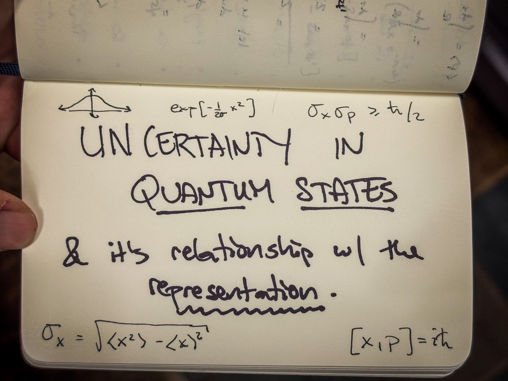
Uncertainty in Quantum States

A preparation for the study of Quantum Coherence

Hey Friends,

We’re closing in on the last few of the Quantum Mechanics themed lectures in representation theory. Of immediate concern are some details around continuous representations of the algebra of operators.

More precisely, we will compare and contrast the physical implications for continuous and discrete representations. We will use the latter in the study of coherent states.

Best,

Sean

---

In Quantum Mechanics, the Hilbert space of physical states of particulate matter may have two qualitatively distinct forms, it may be continuous or discrete¹.

Free Particles and Continuous Hilbert Spaces

Typically, a Hilbert space of physical states is continuous if the domain of the position of the particle is also infinite. Continuous of course means it’s a vector space of uncountably infinite dimension.

This is typical of a free particle - a particle that moves without the influence of an external force².

The Hilbert space of free particles in one-dimension is typically represented by as the function space of solutions graded by the real number, R. For example, we can parametrize the energy of plane waves in one-dimension by the wave number k:

\(\psi_{k}(x) = A \exp\left(ikx - iE_{k}t\right).\)

Plane waves are eigenfunctions of the energy operator

\(E = -\frac{\hbar^{2}}{2m}\frac{d^{2}}{dx^{2}},\)

where

\(E\cdot \psi_{k}(x) = \frac{(\hbar k)^{2}}{2m}\psi_{k}(x) = E_{k}\psi_{k}(x).\)

But plane waves aren’t physically realistic solutions.

The practical problem with a plane wave solution is that the particle represented by one has an equal probability of being found at any value of x. Hence the experimental uncertainty in its position due to Quantum effects is literally infinite.

Whereas, we know its momentum with exact precision. Indeed,

\(P\cdot \psi_{k}(x) = -i\hbar \frac{d\psi_{k}(x)}{dx} = \hbar k\,\psi_{k}(x).\)

In the real world, we can typically measure both position and momentum to some extent. One of the big insights given to us by Quantum Mechanics is that nature bestows upon as a fundamental uncertainty to measuring both of those quantities simultaneously.

Here we parameterize the uncertainty in terms of the standard deviation of possible observations of given operator, using momentum as an example,

\(\sigma_{p} = \sqrt{\langle P^{2}\rangle - \langle P\rangle^{2}}.\)

Of course, we are using Hermitian operators here, which are those that play nicely with the inner product,

\(\langle P \rangle = \langle \psi , P\cdot \psi \rangle = \langle P\cdot \psi ,\psi \rangle = \int dx \; \psi^{\star} P \cdot \psi.\)

The relationship between the uncertainties in position and momentum is codified in the famous Heisenberg Uncertainty Relation, wherein the product of the standard deviation³ of all possible measurements of position and momentum are bounded below:

\(\sigma_{x}\sigma_{p} \geq \frac{\hbar}{2}.\)

Hence it is no surprise that if σp is zero that σx must be infinite to satisfy this bound.

But why are we considering solutions with known momentum?

This is because we are literally parametrizing the Hilbert space of states with momentum. Another way to say that is we have an R-graded Hilbert space of states. This is all a conspiracy of linearity. The plane wave representation essentially affords a Fourier Analysis of a real, physical particle.

This is a problem of our own choosing. We could have alternatively demanded a representation for which x is precisely known.

\(x \cdot \phi_{x}(p) = i\hbar\frac{d\phi_{x}(p)}{dp},\quad p\cdot \phi_{x} = p\,\phi_{x}(p).\)

Of course, these are also plane waves,

\(\phi_{x}(p) \sim A e^{ipx}.\)

These representations confused physicists for a little bit, and resulted in the famous, but silly, wave-particle duality discussions.

The way around this problem - the way to get physically sensible models of a free particle - is to take a linear combination⁴ of Fourier modes, supported over some normalized distribution. This is typically called a wave packet. Schematically one might look like this,

\(\Psi(x,\sigma) = N(\sigma) \int_{\mathbb{R}} dk\; \psi_{k}(x) \exp\left(-\frac{k^{2}}{2\sigma^{2}}\right).\)

Here σ parameterizes the Gaussian function which supports the full wavefunction over the space of possible wave numbers⁵ and hence momenta. The larger σ, the wider the spread.

We see here that σ parameterizes the error in our knowledge of the momentum. One can go on to show that Ψ(x,σ) now has finite uncertainty in both position and momentum⁶, for which σ essentially serves to parametrizes both.

We can therefore use Ψ(x,σ) to model a physical particle moving freely through space and time.

From this perspective, the Fourier modes of the free particle are just an artifact of the representation, and infinite-dimensional vector spaces are arguably just as counter intuitive as Quantum Mechanics.

Taking Fourier Analysis too seriously was understandable in the 1920s. Somehow, a 100 years later, a few people are still struggling with it. I wrote a piece at Physics! about exactly this issue:

There is one last thing, however. The time evolution of Ψ(x,σ) is complicated, as the energy depends on the wave vector, each mode picks up an complex phase,

\(\Psi(x,t) = N(\sigma) \int_{\mathbb{R}} dk\; \exp(ikx - iE_{k}t)\exp\left(-\frac{k^{2}}{2\sigma^{2}}\right).\)

This cause the wave packet to spread out in time, meaning that the uncertainty in position will grow in time, due to this dispersion.

A Sketch of Wave Packet Spreading

To see this, we need only compute this integral. To that end, we first algebraically resort things so that the integral has the form,

\(\Psi(x,t) = N(\sigma) \int_{\mathbb{R}} dk \; \exp(-\alpha k^{2} + \beta k)\)

For some complex numbers α and β. Note that α depends on time and β depends on position. The standard calculation of a Gaussian integral gives

\(\Psi(x,t) = A \exp\left( -\frac{x^{2}}{2\alpha}\right),\)

where A is an overall factor that depends on time and the original gaussian preparation parameters σ. It is scaled so that the function is normalized.

Computing the expectation value of x,

\(\langle x \rangle = \int_{\mathbb{R}} dx\; \Psi^{\star}(x,t) x \Psi(x,t),\)

which vanishes because its an odd integral. Similarly the expectation value of p vanishes. We are then left with,

\(\sigma_{x}^{2} = \int_{\mathbb{R}} dx\; \Psi^{\star}(x,t) x^{2} \Psi(x,t),\quad \sigma_{p}^{2} = -\hbar^{2}\int_{\mathbb{R}} dx\; \Psi^{\star}(x,t) \frac{d^{2}\Psi(x,t)}{dx^{2}}.\)

Both of these integrals are even and non vanishing, and the answers depend on the parameter α, which itself depends on time.

Gory details aside⁷, σx and σp include terms that depend on α, and you can show that both increase with time as the wave packet spreads. At large values of t, the uncertainties effectively grow linearly in time.

Amusingly, the wave packet at time t = 0 saturates the lower bound on the uncertainty relation

\(\sigma_{x}\sigma_{p} =\frac{\hbar}{2}.\)

But of course this product increases away from this lower bound as time progresses.

This is an example of incoherent time evolution, as the individual, linearly independent modes evolve on their own, spreading the wave packet and making our knowledge of the particle’s position and momentum less certain as a function of time.

Bound Particles and Discrete Hilbert Spaces

A discrete Hilbert space typically appears when the particle is bound by a force. The simple harmonic oscillator, whose potential energy can be written as a function of position x,

\(V(x) = \frac{1}{2}m\omega^{2}x^{2},\)

typically restricts the motion of the particle to a domain proportional to the square root of the total energy,

\(E = -\frac{\hbar^{2}}{2m}\frac{d^{2}}{dx^{2}} + \frac{1}{2}m\omega^{2}x^{2} .\)

For the past few lectures we have been studying various representations of this system, some analytic, some algebraic. In terms of the so-called eigenkets.

\(| n \rangle = \frac{1}{\sqrt{n!}} a^{\dagger n} | 0 \rangle.\)

Now what’s interesting about these states is they are already based on the Gaussian function in position⁸. They have finite uncertainty in both position and momentum,

\(\sigma_{x} = \sqrt{\frac{\hbar(2n+1)}{2m\omega}},\quad \sigma_{P} = \sqrt{\frac{\hbar\omega m (2n+1)}{2}}.\)

So physically, these are already pretty well-defined states, and in particular,

\(\sigma_{x}\sigma_{p} = (2n+1)\frac{\hbar}{2}.\)

Now individual eigenstates or kets of the energy operator each have fixed values of energy, so the time evolution of a ket is

\(| n(t) \rangle = \frac{e^{-iE_{n}t}}{\sqrt{n!}}a^{\dagger n} | 0 \rangle,\quad E_{n} = \frac{\hbar\omega}{2}\left(2n+1\right).\)

Unlike the Gaussian wave packets of the free particle, this single energy states are coherent in the sense that σx and σp are constant in time. There is no dispersion. To see this you need only observe that the time-dependence enters only as a complex phase.

TL;DR

Today we explored some qualitative differences between different representations of the basic Heisenberg algebra of quantum mechanics,

\([x,p] = i\hbar.\)

The choice of representation depended strongly on the physical details of the system involved. In particular we compared the continuous, free particle representation with the discrete, harmonic oscillator one.

Next time, we’ll study the Quantum theory of light and show how it utilizes details from both kinds of representations.

1. We’ve said this before, but for the aficionados out there, this distinction happens with representations of Lie algebras all the time. More on this later / keep your eye on this space.

2. In realistic physical systems we often model the potential energy as a piecewise smooth function, so there is some nuance in the form of stitching together individual neighborhoods of physical phenomena. For example, a particle may be free for all x greater than some fixed number, after which it experience a potential. There are some global considerations present in the sense of quantum tunneling, although those solutions are typically also realized as boundary value problems. That said, tunneling can connect between discrete and continuous representations, where a meta-stable configuration decays into a free particle that runs away to infinity. This is a distinctly quantum phenomena, but this is beyond the scope of our little introduction to representation theory.

3. This assumes that whatever the probability distribution is obeys the assumptions of the central limit theorem. This is implicit in the definition of the state of quantum mechanics. For practical purposes here the standard deviation of an operator’s spectrum is the square root of the ( variance minus the square of the mean ).

4. Remember, the space of physical states is a vector space, so we can of course consider states that are linear combinations.

5. In one dimension, a wave vector is but a number, but it is still 2π/λ, with λ being the wavelength.

6. Just do the integral. The Fourier transform of a Gaussian is a Gaussian. Not only it offer finite uncertainty in position and momentum, but the choice of a Gaussian function to support the momentum ( or the position ) results in a quantum state that has the minimum possible uncertainty in their product. Explaining this would take us pretty far afield into the Heisenberg Uncertainty Principle Quantum Mechanics.

7. See this useful integral chart for help doing these calculations yourself.

8. We alluded to this briefly in our first lecture on the harmonic oscillator. These are Gaussian functions multiplied by the Hermite polynomials:

The Physical Origins of Heisenberg Algebras